You’re an investigator — let’s you receive a call from a museum to solve the robbery of a priceless piece of art. But footage is missing, footprints and fingerprints are not complete, and witness testimony is not the most reliable. I will go through this process to explain an important algorithm for missing data:

Figure 1 – The unsolved 1990 Gardner Museum Heist
You rush home, put together your board:

- You start with what you already have and fill-in the blanks:
- A ssmudged footprint by the display-case
- Surveillance footage that cuts out half-way
- A broken window by the painting
You assume that:
#1 The criminal entered at 2.a.m when the camera cut off
#2 They left through the broken window by the painting.
The MICE algorithm starts with random assumptions as placeholders for missing data.
2. You focus on 1 missing piece – the getaway time:
You are able to check:
- Sensor data of people leaving and entering other rooms.
- Cleaning crew logs
- Patterns from similar break-ins
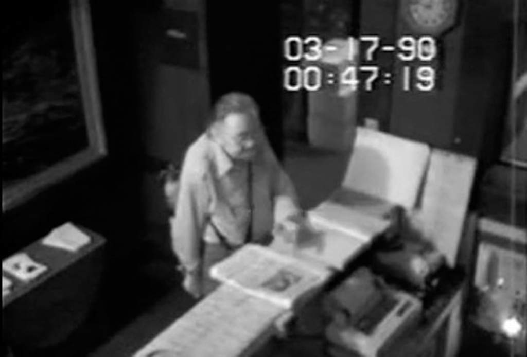
Figure 2 – Footage from the unsolved 1990 Gardner Museum Heist
MICE uses a model to impute (estimate) one variable using all the others in the dataset. The original guess of leaving was 2:30am, but with this other data, you update this time to 3:15 am based on other sensor activity and patterns from other similar break-ins.
The missing value in MICE is now filled with a smarter, imputed (estimated), data-informed prediction.
3. Do it again, but with another clue – smudged footprint by the display-case
You are able to check:
- Stride length
- Clear size 12 footprint in room next door
- Pressure marks on the footprint
You are then able to tell the weight and shoe size of the suspect.
MICE moves to the next variable and imputes its value based on this new state of the dataset.
4. Loop through the scene again
You revisit the entire scene again, with new data.
5. Build several stories:
- Thief uses East exit.
- Paused near the staff lounge
Each version is slightly different.
MICE generates multiple datasets with different imputation paths to reflect uncertainty.
6. Compare versions to find consistent truths
You analyze the different reconstructions to find stable details — shoe size, exit time.
MICE pools results from all datasets to produce less biased estimates
You are then able to narrow your suspects down significantly.
Technically, it looks like this:
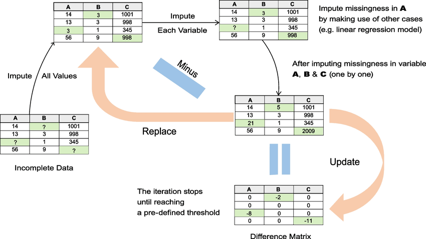
Figure 3 – Ke et al (2022)
- Incomplete data
- Random value in incomplete spaces across all columns
- Focus on one column at a time — say A. Remove all guessed values from A, using other columns — build an AI model that learns how the other columns (B and C in this case) relate to A.
- Do the same for all other columns (B and C).
- “Minus” subtract the old guesses from the new ones. This indicates how much learning there is left to do.
- Update (replace with new values).
- Loop
A fun metaphor for this:
Think of your data like a Swiss cheese sandwich — full of holes.
MICE fills those holes by looking at the rest of the sandwich, one slice at a time. It keeps layering and re-smoothing until the sandwich looks whole again.
This is very very real — in long-term studies, such as the 2011 study by Enders, in which participants where expected to give 3 depression assessments over the course of 3 months. Where only 71.4% of participants had complete data across all time points. The remaining 28.6% had at least one missing data point.
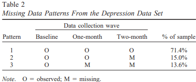
Figure 4 – Enders (2011) — (O= observed, M= missing)
So maybe consider MICE when given incomplete data.
Sources:
Enders, C. K. (2011). Analyzing longitudinal data with missing values. Rehabilitation Psychology, 56(4), 267–288. https://doi.org/10.1037/a0025579
Ke, X., Keenan, K., & Smith, V. A. (2022). Treatment of missing data in Bayesian network structure learning: An application to linked biomedical and social survey data. BMC Medical Research Methodology, 22(1), Article 281. https://doi.org/10.1186/s12874-022-01781-9
